|
<< Click to Display Table of Contents >> Meridional flow calculation |
  
|
|
<< Click to Display Table of Contents >> Meridional flow calculation |
|
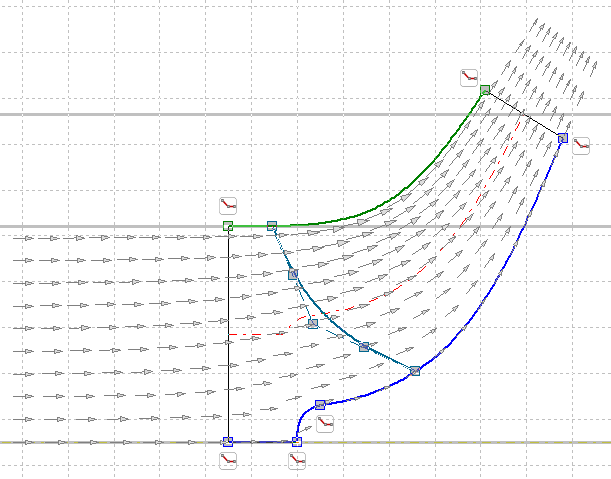
Meridional flow visualization based on potential flow theory is available optionally. The result of meridional flow calculation can be displayed using the button top right of the diagram. ![]()
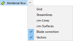
The display can be configured using the corresponding menu (all options can be combined).
|
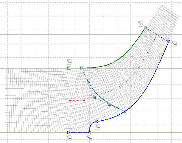
Grid After each change of the meridional contour a new computational grid is calculated. Extensions are added to the inlet and outlet in order to ease the setup of the boundary conditions.
|
|
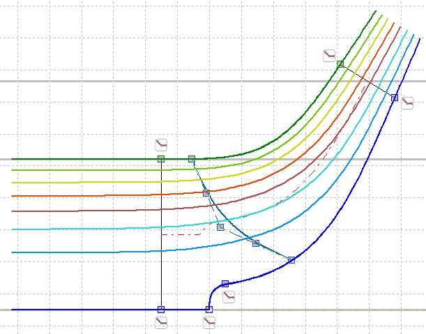
Streamlines meridional streamlines (lines with constant values of the stream function) equal mass flow fraction between neighboring streamlines |
|
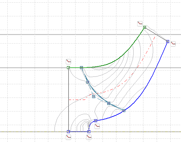
cm-lines iso lines of const. meridional velocity cm |
|
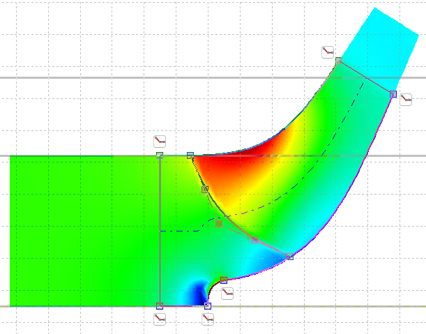
cm-surfaces iso surfaces of const. meridional velocity cm (scaling is displayed below the diagram) |
Blade correction If activated, the blockage effect of blade thickness is considered for flow calculation. |
|
|
Vectors vectors of meridional velocity cm |
Within the meridian the equation for stream function ψ will be solved. For an incompressible fluid this equation is in cylindrical co-ordinates (z, r):
.
For a compressible fluid the equation looks like:
.
where a is the sonic speed defined by:
.
Hub and shroud are representing stream lines where as at in and outlet there is a certain stream function distribution chosen. This is done in accordance to the mass flow imposed by the global setup.
The equation is solved using a finite-difference-method (FDM) on a computational grid, which will be generated using an elliptic grid generation. For more information about the used computational techniques refer to e.g. Anderson et al.
The meridional velocity component can be calculated by the axial velocity component:
.
by the radial velocity component:
.
with:
.
rR and ρR are reference radius and density respectively. In case of incompressible fluids the density is constant throughout the flow domain and the according term in the equations is discarded.
Due to the potential flow theory the given solution is only a rough estimation of the real meridional flow. One has to bear in mind that friction is not considered as well as the no slip boundary condition at hub and shroud. For detailed flow analysis CFD-techniques for solving the entire set of Navier-Stokes-Equations has to be used. Also the solution scheme implemented (FDM) may not always find a solution for every combination of design point and meridional contour.
Singularities will occur if the solution domain has radii close to zero. Then at those locations some artefacts might exist in the meridional velocity contours.
For compressible fluids it is necessary that the flow regime in the entire domain has to be far away from transonic conditions. Otherwise the equation will not have solution.