|
<< Click to Display Table of Contents >> Blade-to-blade flow 2D |
  
|
|
<< Click to Display Table of Contents >> Blade-to-blade flow 2D |
|
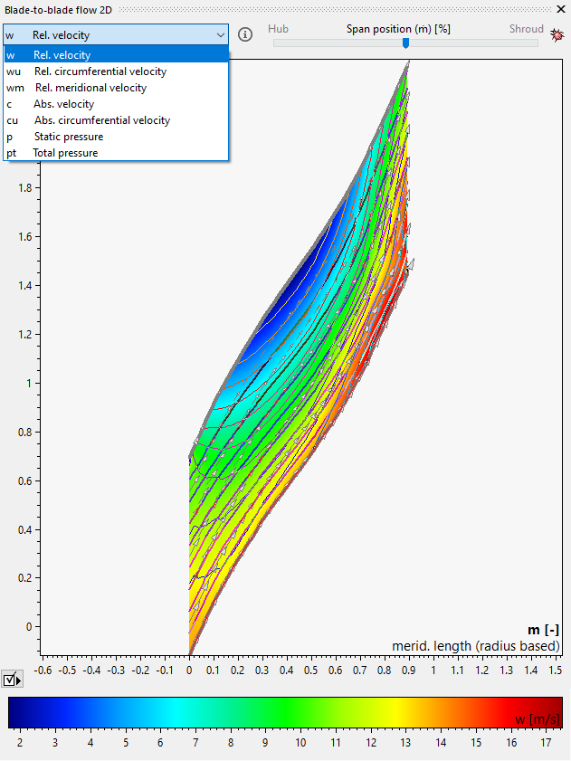
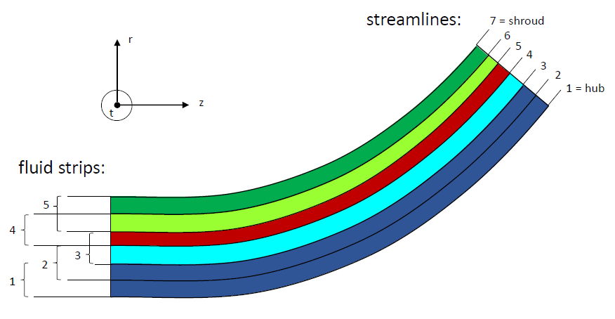
Stream lines must be known a-priori (see Meridional flow calculation). If the meridional flow calculation failed, blade-to-blade flow 2D cannot be calculated and the diagram will not be available. The stream lines rotated around the z-axis build stream surfaces.The relative stream function and relative velocities will be calculate in a blade-to-blade section, that is encapsulated by two stream surfaces and represent a fluid strip. Since hub and shroud are considered as stream lines, there are always two fluid strips less than stream lines. All calculations of the relative stream function and its derivatives are done within a fluid strip that has a stream surface in between. Results of these calculations are given for fluid strips that correspond to inner stream lines or surfaces resp. In the picture below those stream lines have indexes from 2 .. 6.
In contrast to the Stanitz&Prian approach here a two-dimensional relative flow is calculated. This equation in m-t co-ordinates reads as:
![]() .
.
This equation can be derived from the the assumption of zero absolute rotation of the flow in the fluid strip between two adjacent blades and from the equation of continuity in two dimensions respectively:
![]() ,
,
![]() .
.
Here w is the relative velocity, ω is the rotational speed and ρ is the fluid density. In the equation above Δn is the normal height of the fluid strip. Another assumption is that there is no variation of the density with respect to the tangential co-ordinate t. The information about the meridional distribution is coming from the Stanitz&Prian approach.
The boundary conditions are defined as follows. At the suction side a stream function value of zero is set whereas at the pressure side it is set to the mass flow that is conveyed through the fluid strip. For the 5 fluid strips this is 2/5 times the design point mass flow.
![]() ,
,
![]() .
.
At inlet and outlet all stream function values are linearly interpolated with respect to the tangential co-ordinate t. Then all stream function values are defined at the boundaries.
The equation is solved using a finite-difference-method (FDM) on a computational grid, which is generated by interpolating mean lines between pressure and suction side. For more information about the finite-difference-method refer to e.g. Anderson et al.
The tangential and the meridional relative velocity component resp. can be calculated by:
![]() ,
,
![]() .
.
The static pressure pi can be determined by using the constancy of the rothalpy. For incompressible fluids that reads:
![]() .
.
For compressible fluids the same principle is applied for the specific enthalpy and temperature resp. with the assumption of perfect gas behavior. Since the density is already known the static pressure can be calculated using the equation of state p=f(T,ρ).
![]() .
.
The total pressure is derived from the Bernoulli equation for incompressible fluids and by assuming an isentropic state change from (p,T,c>0) -> (pt,Tt,c=0) for compressible fluids.
[ Compressors and Turbine rotors only ]
Mach Number can be displayed both relative as well as absolute.
![]()
![]()
Here a is the sonic speed defined by:
![]()
The specified mass flow can only be realized for a certain size of the cross section at the given total inlet state. If the combination of mass flow, total inlet condition and geometry (cross section) yields a state that is physically not possible a solution cannot be determined and a hint is displayed saying: "No solution due to shocks, transsonic behavior or numerical reasons at span: x". x will hold the actual span number for which the hint is true.